Electrical Resistivity Sounding and Tomography Services
Electrical resistivity tomography emerged from early studies on the electrical resistivity properties of rock, soils, and fluids. The theory and principals are well defined using two to four electrodes to measure the subsurface properties. As a result, one can find references to studies going back to the 1920’s. Before computer controlled switching systems became available, it was nearly impossible to collect a large volume of electrical resistivity data in a reasonable amount of time. Once that obstacle was overcome, computer software emerged allowing enormous amounts of data to be processed and inverted. The results were impressive. Consequently, near surface geophysical surveys using electrical resistivity methods focused on characterizing soils, types of rock, formation thickness, fracturing, jointing, faulting, contamination, delineating fill, finding voids, and mapping large scale geologic features.
How does electrical resistivity tomography work
The basic premise for electrical resistivity surveys relies on the concept that the ground responds like a group of electrical resistors. Thus, by injecting a current into the ground one can measure the potential difference between two points. Consequently, one may create an infinite number of combinations and permutations for the placement of the current electrodes and the potential electrodes. On the other hand, there are only a small number of user-friendly geometries. For example, the majority of resistivity surveys use dipole-dipole, Wenner, Schlumberger, pole-dipole, and pole-pole arrays. Each one of these arrays offers a unique response. Some are better at mapping lateral variations, while others more accurately estimate the depth of geologic units or are capable of reaching greater depths of penetration.
Electrical Resistivity Imaging Theory
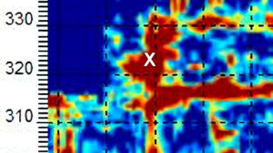
Fundamentally, as one expands the distances between electrodes about a center point, the resistivity equipment is responding to a greater bulk volume of material from greater depths. If one repeats this process by moving the center point along a line, an operator would have electrical resistivity data that reflects the apparent resistivity as a function of apparent depth or pseudodepth. These results create a pseudosection. The pseudosection by itself has value but is difficult to interpret. Yet, by creating computer generated geologic models that approximate the response measured in the field, one has a method for characterizing or visualizing the conditions at depth along a line. The process of acquiring and processing electrical resistivity data in this manner is electrical resistivity tomography or electrical resistivity imaging.
To sum it up
Electrical resistivity tomography works by collecting thousands of apparent resistivity values along a line. In addition, by increasing the spacing of the electrodes, about a center point, the electrical resistivity data reflects changes at depth. A computer program like AGI’s EarthImager or M. H. Loke’s RES2DINV software imports the electrical resistivity data and processes it. The processed results yields one or more models that represent the geology or conditions at depth along the line. In the same way groundwater modeling predicts non-unique models for groundwater flow, permeability, and hydraulic conductivity, electrical resistivity tomography cannot produce unique results. Unlike groundwater modeling, which seldom has a large database field values to work with, thousands of apparent resistivity values go into creating an electrical resistivity imaging model. By combining different types of arrays, one can easily acquire four to five thousand data points along a single resistivity line.
Electrical resistivity tomography method
DC resistivity or traditional galvanically coupled resistivity methods
First, one needs to determine the objective of the electrical resistivity survey. One needs to ask, “Is the objective to map lateral variations or is it more important to differentiate changes in unit or formation thickness? Is the depth of investigation tens of feet or hundreds of feet?” Answers to these questions assist with determining what type of array to use (e.g. Wenner, dipole-dipole, Schlumberger, or other). Furthermore, if one is looking to observe the transient response or decay of injected current, one may want to consider a dipole-dipole arrays for conducting an induced polarization or IP survey.
What type of electrical resistivity array to use
H. Loke points out the following: If your survey is in a noisy area and you need good vertical resolution and you have limited survey time, use the Wenner array. If good horizontal resolution and data coverage is important, and your resistivity meter is sufficiently sensitive and there is good ground contact, use the dipole-dipole array. If you are not sure, or you need both reasonably good horizontal and vertical resolution, use the Wenner-Schlumberger array with overlapping data levels. If you have a system with a limited number of electrodes, the pole-dipole array with measurements in both the forward and reverse directions might be a viable choice. For surveys with small electrode spacings and good horizontal coverage is required, the pole-pole array might be a suitable choice.
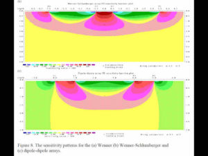
Electrical Resistivity Sensitivity Pattern by M.H.Loke
Where is a good place for an electrical resistivity imaging survey
Secondly, one needs to find a reasonable location to conduct an electrical resistivity tomography survey. Be aware that extreme topographic changes or rapid changes in direction along a line can compromise the survey. While EarthImager and RES2DINV can take into account the effects of rapid changes in geometry, it is not always clear how well these adjustments reflect extreme conditions. At the same time, one may want to consider if the acquisition of parallel or perpendicular resistivity lines will lead to a more definitive interpretation. As a minimum, these additional lines offer redundancy that improve confidence.
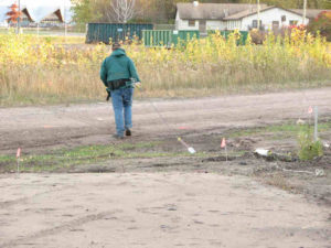
How is a electrical resistivity imaging survey conducted
Finally, after the objective is determined, the type of resistivity array is decided on, and a suitable location is found, one can conduct an electrical resistivity tomographic survey. While one can find specific details about electrical resistivity equipment below, the following is a general idea of what takes place using an AGI 84 electrode SuperStingR8 system. The multi-electrode electrical resistivity system is flexible enough to handle 28 to 168 electrodes. It is common to use 56 to 84 electrode configurations. An 84 electrode array with electrodes spaced five meters apart can reach depths in excess of two hundred feet. At the same time, the amount of line covered at these greater depths of penetration is much less than the amount of line covered near the surface.
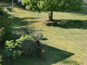
Electrical Resistivity Imaging Tomography
To sum it up, the electrical resistivity instruments are setup at the center of a resistivity line. The instruments include the main SuperSting R8 console, an 84-channel switch box, and one or two deep cycle 12VDC batteries. The SuperSting console, for most near surface geophysical applications, is both the transmitter and the receiver. Once the instrument is setup, the operator lays out two sets of cables in a straight line, which extend out in opposite directions from both sides of the SuperSting. As a result, each set of cables has 42 take outs or places to connect electrodes on each side of the SuperSting. At each take out, an electrode is placed in the ground at the desired spacing. To decrease the contact resistance between the electrodes and the ground, a field person may pour water on the ground at each electrode.

Capacitance coupled resistivity methods
Unlike galvanic coupled or DC resistivity equipment, discussed above, Geometrics designed and builds a geophysical instrument that does not require electrodes. The electrical resistivity system, called an OhmMapper, produces an alternating current in the subsurface with a transmitting alternating high voltage dipole. The alternating high voltage transmitter couples with the subsurface in the same fashion that a capacitor functions. The capacitance coupled transmitted alternating current flows through the subsurface and couples with the receiver, creating a measurable voltage. The results duplicate the response of a dipole-dipole array with a SuperSting.
While the OhmMapper is not likely to reach the depths of investigation that the AGI multi-electrode resistivity imaging system is capable of, the OhmMapper is fast and portable. By dragging the OhmMapper across the ground using different dipole configurations, one can acquire electrical resistivity tomography data. M. H. Loke’s RES2DINV software works well to process the OhmMapper results. One great benefit of this system is that an operator can pull it across hundreds of acres. Consequently, one can map variations in apparent resistivity across an entire site. A plan view contour plot of apparent resistivity often assists with locating areas of concern. These areas of concern can then be detailed with an electrical resistivity imaging survey. Though the results reflect changes in apparent resistivity, it is an excellent alternative to Geonics EM31, EM34, or EM38, which does not always work well in electrically resistive soil conditions.
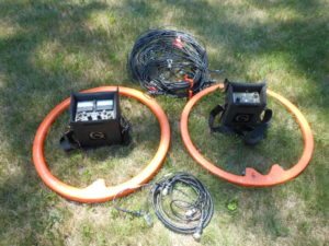
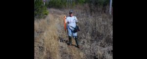
Electrical Resistivity Capacitance Coupled Towed Array
Electrical resistivity tomography depth
The depth of investigation for an electrical resistivity imaging survey is a function of the total length of the array. Different resistivity arrays offer different depths of investigation. For instance, a standard Wenner array (per M. H. Loke) has a median depth of penetration of approximately 0.173 times the total array length. However, dipole-dipole arrays have a set of values that correlate to its N spacing (a ratio associated with the geometry of the dipole-dipole setup). Thus, a standard dipole-dipole array (per M. H. Loke) with an N of 1 has a median depth of penetration of approximately 0.139 times the total array length, while an N of 3 offers a median depth of penetration of approximately 0.192 times the total array length.
Although the maximum depth of penetration is dependent on the instrumentation, subsurface conditions play an important role. The unit or formation thickness and its absolute resistivity values influence the measured apparent resistivities. It is not until the data is inverted or modeled that one can get a feeling for the true approximate depth of investigation. Unlike DC resistivity surveys, the OhmMapper has limits associated with how it capacitively couples with the subsurface. The greatest depths of investigation will be obtained over materials with high electrical resistivity values. Conductive clay rich soils and water are not well suited for an OhmMapper survey. Because the OhmMapper responds as a dipole-dipole array, the electrical resistivity tomography depth is the same as for the SuperSting system.
Electrical resistivity tomography equipment
Summary of Geometrics OhmMapper specifications (details from Geometrics)
The OhmMapper consists of the transmitter electronics and batteries along with two transmitting dipole cables. The transmitter is towed via the nonconductive tow link connecting it to the receiver. The receiver consists of the transmitter electronics, batteries, and dipole cables. The receiver voltage level is converted to a digital signal in the receiver and transmitter to the data logger worn by the operator. The operator carries the data-logging console (DataMapper) at his waist.
The new Geometrics OhmMapper is a capacitively coupled resistivity meter that measures the electrical properties of rock and soil without cumbersome ground stakes used in traditional resistivity surveys. A simple coaxial-cable array with transmitter and receiver sections is either pulled along the ground by a single person or attached to an all – terrain vehicle. Data collection is many times faster than systems using conventional DC resistivity.
High Speed Capacitively-Coupled Resistivity System
Features:
Full dipole-dipole resistivity profile can be done in a fraction of the time taken for traditional resistivity measurement. Operates over frozen ground, ice, concrete, and other areas where grounded dipole measurements are difficult to make. Data is logged to Geometrics DataMapper logging console for easy tracking and positioning of resistivity data. Post acquisition processing is facilitated with Geometrics DataMap software for editing of data, positioning of data, and creating output compatible with third-party mapping and processing software.
Specifications:
Operating principle: Constant-current capacitively-coupled, dipole-dipole resistivity
Operating range: Less than 1 OhmMeters to greater than 100,000 OhmMeters
Cycle Rate: Signal sample and data logging rate at 2 times per second
Transmitter specifications:
Frequency under 18 kHz
Output current: variable from 16 mA to 0.25 mA
Receiver Specifications:
Dipole lengths: 5 m, 10 m, 15 m, 20 m, longer lengths optional
Survey Types:
Continuous, constant-offset dipole-dipole resistivity. (Multi-line with constant transmitter-receiver spacing for plan-view mapping.)
Variable-offset, dipole-dipole resistivity. (Variable transmitter-receiver spacing for multiple passes on a single profile line to create a pseudosection.)
Summary of AGI’s SuperSting R8 electrical resistivity system specifications (details from AGI)
AGI’s multi-electrode electrical resistivity imaging system consists of the SuperSting R8 console, interconnect cables, a passive switch box for addressing electrode locations, two forty-two take out cables (each divided in to three sections), and 84 stainless steel stakes or pins. The 12VDC batteries provided by the user power the system. Software and cables allow data transfer to a PC. Post processing is typically accomplished using AGI’s EarthImager software, which is user friendly with the system.
Description:
Measurement Modes: Apparent resistivity, resistance, induced polarization (IP), SP, and battery voltage.
Measurement Range: +/- 10Vp-p.
Measuring Resolution: Max 30 nV—depends on voltage level.
Screen Resolution: 4 digits in engineering notation.
Transmitter: 200W internal transmitter. 5kW, 10kW and 15kW external transmitters also available (see separate brochure).
Output Current: 1 – 2000 mA continuous, measured to high accuracy.
Output Voltage: 800 Vp-p—actual electrode voltage depends on transmitted current and ground resistivity.
Input Channels: 8.
Input Gain Ranging: Automatic—always uses full dynamic range of receiver.
Input Impedance: >150 MOhm.
SP Compensation: Automatic cancellation of SP voltages during resistivity measurement. Constant and linearly varying SP cancels completely (V/I and IP measurements).
Type Of IP Measurement: Time domain chargeability (M). Six time slots measured and stored in memory.
IP Current Transmission: ON+, OFF, ON-, OFF. IP Cycle Times: 0.5, 1, 2, 4, and 8 s.
Measure Cycles: Running average of measurement displayed after each cycle. Automatic cycle stops when reading errors fall below user set limit or user set max cycles are done.
Resistivity Cycle Times: Basic measure time is 0.2, 0.4, 0.8, 1.2, 3.6, 7.2, or 14.4 s as selected by user via keyboard. Autoranging and commutation adds about 1.4 s.
Signal Processing: Continuous averaging after each complete cycle. Noise errors calculated and displayed as percentage of reading. Reading displayed as resistance (dV/I) and apparent resistivity (ohmm or ohmft). Resistivity is calculated using user-entered electrode distances.
Noise Suppression: Better than 100 dB at f >20 Hz. Better than 120 dB at power line frequencies (16 2/3, 20, 50, and 60 Hz) for measurement cycles of 1.2 s and above.
Total Accuracy: Better than 1% of reading in most cases (lab measurements). Field measurement accuracy depends on ground noise and resistivity. Instrument will calculate and display running estimate of measuring accuracy.
System Calibration: Calibration is done digitally by the microprocessor based on correction values stored in memory.
Supported Configurations: In manual mode: Resistance, Schlumberger, Wenner, dipole-dipole, pole-dipole, and pole-pole.
In automatic mode: Any configuration can be programmed via command file.
Operating System: Stored in reprogrammable flash memory. Updated versions can be downloaded from our website and stored in the flash memory.
Data Storage: Full resolution reading average and error are stored along with user-entered coordinates and time of day for each measurement. Storage is effected automatically in a job-oriented file system.
Data Display: Apparent resistivity (ohmmeter), current intensity (mA), and measured voltage (mV) are displayed and stored in memory for each measurement. Data can also be displayed on an Android device in real time as bright color pseudosections, IP curves, transmitter/receiver plot, contact resistance measurements, and more.
Memory Capacity: The internal SuperSting memory can store more than 79,000 measurements (resistivity mode) and more than 26,000 measurements in combined resistivity/IP mode.
Data Transmission: Data can be instantaneously transferred from the Android device by email or by file transfer from the Android device USB port. RS-232C channel available to dump data from instrument to a Windows-type computer on user command.
Automatic Multi-Electrodes: The SuperSting is designed to run dipole-dipole, pole-dipole, pole-pole, gradient, Wenner, and Schlumberger surveys including roll-along surveys completely automatic with the patented Dual Mode Automatic Multi-Electrode system (U.S. Patent ,404,203) or a passive electrode cable system.
The SuperSting can run any other array by using user-programmed command files. These are ASCII files that can be created using a regular text editor. The command files are uploaded to the SuperSting RAM memory and can at any time be recalled and run as a survey.
Power Supply, Field: 12V or 2x12V DC external power—connector on front panel.
Optional AC/DC power supply and motor generator.
Power Supply, Office: DC power supply.
Operating Time: Depends on survey conditions and size of battery used. Internal circuitry in auto-mode adjusts current to save energy.
Operating Temperature: -5 to +50°C.
Weight: 10.9 kg (24 lbs.).
Dimensions: Width: 184 mm (7.25″). Length: 406 mm (16″). Height: 273 mm (10.75″).
Locating Deep Facilities Using ERI, EM, MASW, pulseEKKO Ultra GPR, and Magnetometers for Buried Cables Voids Pipes
Geophysics for voids under buildings, floors, foundations, parking lots, and factories
Geophysical Services Conducted. A Short List of Clients, Landfills, Government Sites, and Locations.

Chart Comparing 57 Geophysical Methods With 17 Applications and Disciplines
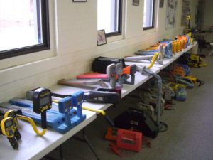
Less Common Near Surface Geophysical Equipment

NAICS and SIC Codes for Geophysical Surveying and Mapping Services
Geophysics and Geophysical Services From Archives and Old Posts