Geophysical services and equipment for investigating shallow bedrock
Today’s discussion on agricultural geophysics focuses on geophysical applications for mapping variations in depth to shallow bedrock and changes in soil and bedrock conditions, which may lead to preferential paths for fluid flow. First, I must point out that much of what I am going to discuss is based on my experiences and reflects my opinions. While the laws of physics behind the geophysical methods are well defined and entrenched in theory, the problem for us, is whether or not we can understand and properly interpret the acquired results. The equipment responds to the earth. We do not always understand or appreciate what we are being told.
Agricultural geophysics covers a range of applications. For example, uses include soil characterization, locating tile lines, mapping private lines, identifying conditions impacted by stray voltage, converting farmland to a mine, and investigating environmental issues. Mining for frac sand, sand and gravel, or crushed limestone is profitable and is becoming more common in rural areas. Locating tile lines, lost private lines (e.g., cables and pipes), or buried well casings is a common use for geophysical methods. Characterizing site conditions with stray voltages is a less common application and potential a more complex study. Here are links to two guides on stray voltage (09-DJR-Stray-Voltage-Field-Guide or Stray Voltage Guide MREC 120917). Without doubt, I suspect a number of you are familiar with using electromagnetic instruments, like a Geonics EM38, to map variations in top soils. Here are two papers on the use of electromagnetic methods for farming (Geonics List of Papers on Agriculture Studies and USE OF ELECTROMAGNETIC INDUCTION TOOLS IN SALINITY ASSESSMENT/APPRAISALS IN EASTERN COLORADO).
Basic geophysical concepts
Only under unique conditions, can one lean on one geophysical method to yield desirable results. A phased approach that integrates two or more geophysical methods can assist with more clearly identifying zones of interest and reduces the chance of false positives or false negatives. If variables like homogeneity, saturation, pore fluid conductivity, and the types of materials are known, then one can focus on limiting the geophysical investigation to fewer geophysical methods. Moreover, we must ask ourselves if it is reasonable to use geophysical methods to characterize what we are investigating. We must decide if what we are looking for is large enough to detect using geophysical methods. At the same time, there must be a detectable contrast between the target and the surrounding area.
To illustrate, attempting to map a shallow bedrock depression that is tens of feet in width and a few feet deep at a depth of five to ten feet is far more likely than if it is covered by a hundred feet or more of soil. Furthermore, if one attempted to map the shallow bedrock depression using electrical methods and the depression was covered by dry clean sand, it is very possible that there would not be a large enough electrical contrast between the rock and the sand to produce good results. On the other hand, if one used seismic methods it is likely that the velocity contrast between the sand and the shallow bedrock is great enough to map the feature.
Geophysical equipment for shallow bedrock investigations
There are two major groups of near surface geophysical equipment. The first group either maps lateral variations over spatially large areas or along transect lines. The second group characterizes changes as a function of depth within a borehole. Without doubt, borehole geophysics utilizing optical borehole imaging tools, temperature sensors, flow meters, EM conductivity meters, and calipers play an important role in characterizing a site. However, I will concentrate on surface geophysical methods, which pertains to the first group.
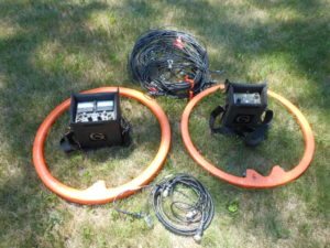
Here is a list of equipment that is often used to investigate the top thirty feet. Electromagnetic instruments include Geonics EM38, EM31, and EM34. I find these instruments well suited for mapping lateral variations across a site. Electrical resistivity tomography or imaging using AGI’s SuperStingR8 with 84 electrodes is an excellent tool for mapping variations along a transect line. An alternative to the SuperSting R8 is Geometrics OhmMapper. Given that it has two modes of operation it can quickly cover spatially large areas or image the subsurface along a transect line. Seismic refraction, MASW, and seismic reflection methods provide considerable detail along a transect line using a Geometrics Geode or GeoStuff’s AnySeis seismograph with 24 to 48 geophones that range from 2 Hz to 40 Hz. Ground penetrating radar works very well if there is little to no top soil, ground water is below its depth of penetration, or the overburden is not electrically conductive (e.g. sand and gravel).
Geophysical methods for characterizing depth to rock or overburden thickness
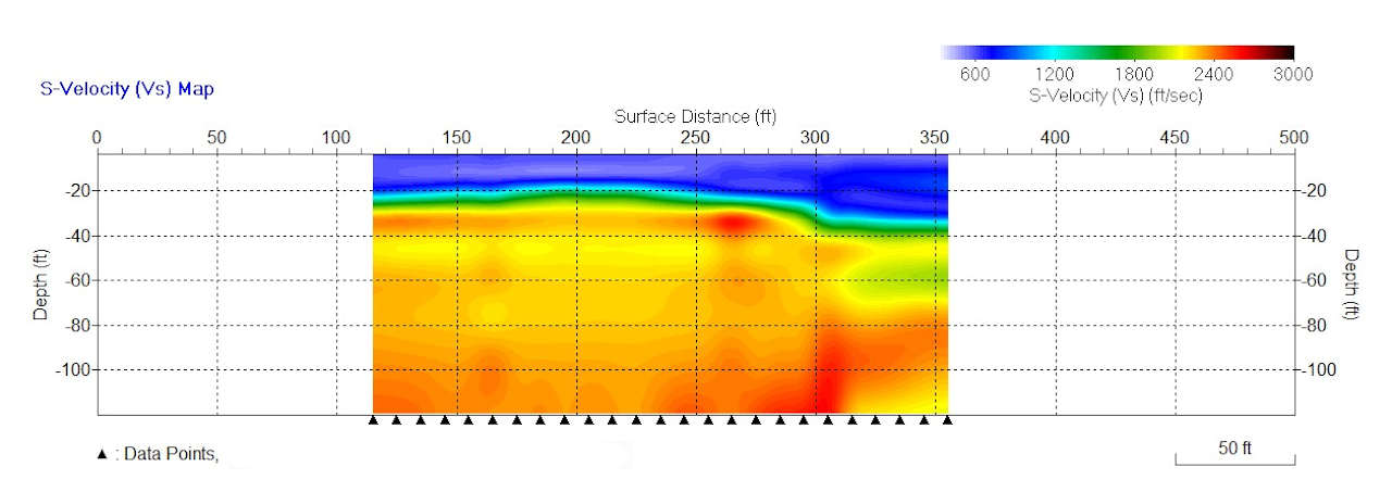
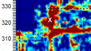
Characterizing the overburden thickness or depth of rock is fairly straightforward, for depths less than about fifteen feet. For depths greater than fifteen feet, one may find multiple geologic units and experience complications associated with the presence of groundwater. These added variables potentially increase the complexity of the final interpretation. One must also consider the level of detail needed to yield desirable results. Attempting to map, more or less, flat lying shallow bedrock is often less of a challenge than mapping local variations in the shallow bedrock topography or weathered zone. Below is a cross-section created from the multi-channel analysis of surface waves or MASW. Its greatest benefit is that it responds to changes in the stiffness of materials and is nearly unaffected by challenges associated with groundwater.
MASW Results for Shallow Bedrock
Interpretation of MASW results
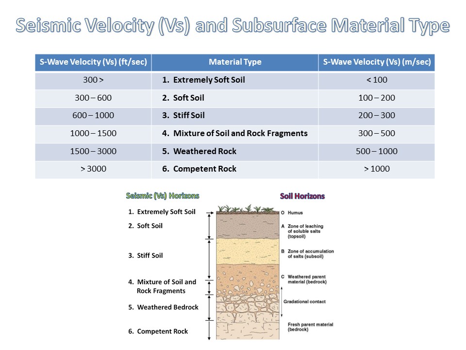
The plot provides an estimate of the overburden thickness and an indication of the competency or potential weathering of the shallow bedrock unit. This analysis is based on the mapped variations in shear wave velocities as a function of depth along the MASW line. Given that there are numerous institutions that classify types of soils and rock formations based on shear wave velocities, one can feel reasonably confident in the MASW approach. Below is a guide by Choon Park of Park Seis, a pioneer of MASW. His presentation is consistent with other charts. He shows that below about 1000 feet per second one is detecting soils. Whereas, shear wave velocities greater than 3000 feet per second indicate competent rock. While between 1000 and 1500 feet per second one may find a mix of soils and rock, less competent types of rock are likely between 1500 and 3000 feet per second.
MASW Soil Classification from Choon Park of ParkSeis
As for the MASW cross section above, one can now interpret the results based on the classifications provided in the chart. In the cross-section it appears that the overburden thickness increases from about 20 feet at station 225 to about 40 feet near station 350. In addition, there appears to be a slight reduction in the shear wave velocities of the shallow bedrock at a depth of 60 feet, near station 325. An interpretation suggests the decrease in velocity may be associated with a decrease in the competency of the shallow bedrock.
Mapping shallow bedrock depressions and valleys
Undoubtedly it requires a greater effort to map small bedrock depressions and valleys then estimating the average depth to rock. So that one can achieve a relatively high level of confidence that a shallow bedrock depression or valley is delineated, data must be closely spaced. In other words, there must be enough data points to avoid false positives or false negatives. The most basic rule suggests that one needs to acquire data at a spacing that is one half the distance of the smallest feature you are looking to map. In my experience, I prefer to see several points along one or more lines. If one keeps this in mind, electromagnetic, electrical resistivity, and seismic methods frequently produce good results for mapping shallow bedrock depressions and valleys.
Seismic refraction for mapping shallow bedrock depressions and valleys
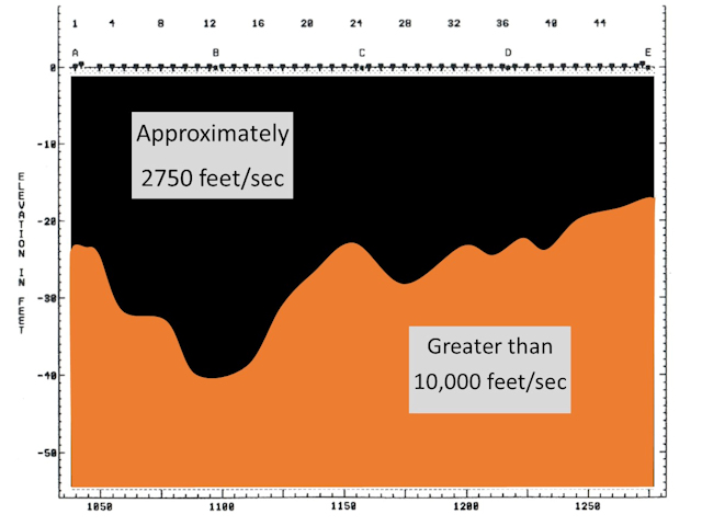
Below is an example of a seismic refraction survey. It was chosen because of the noticeable amount of relief on the shallow bedrock surface. Along the top of the plot the small squares indicate the placement of geophones, which are five feet apart. The total length of the line is 235 feet. Unlike the MASW survey, seismic refraction surveys yield P wave velocities, which are roughly three times faster than shear wave ( S Wave ) velocities. As one can see in the refraction results, the upper area colored in black is overburden. The deeper zone colored in orange represents shallow bedrock. Near station 1100 the overburden reaches a maximum thickness of about 40 feet, which indicates a local depression. As one can see, seismic refraction is an excellent method for mapping the top of rock.
Shallow Seismic Refraction Line
OhmMapper apparent resistivity surveys for mapping shallow bedrock
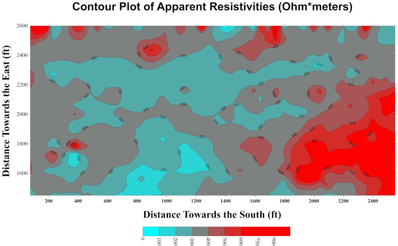
Electrical methods are another good way to map variations in overburden thickness. There are two general types of electrical methods, electromagnetic terrain conductivity surveys and electrical resistivity profiling. While under the topic of detecting preferential paths there is an example of a 1350 acre Geonics EM31 survey, below is a plot showing the results from an OhmMapper survey. This plot represents about 75 acres of a 150 acre investigation. Unlike seismic or electrical resistivity imaging surveys that yield actual depths, electrical profiles measure the apparent conductivity or apparent resistivity of a bulk volume of material beneath the instrument. In general, assuming the soils are homogeneous and the water table is well below the top of rock, apparent resistivities increase with a decrease in overburden, especially with clay rich soils.
OhmMapper Apparent Resistivity Bedrock Map 75 Acres
This plot maps out lateral variations in apparent resistivity. The data was acquired with a towed array using an OhmMapper capacitance coupled electrical resistivity meter. When looking for shallow bedrock, one would look for increases in apparent resistivity. For example, there is a significant increase in the apparent resistivities shown in the bottom right corner of the plot. Bedrock was very close to the surface in this region.
Geophysical methods for identifying preferential paths for fluid to flow within a geologic unit.
Unlike shallow bedrock surveys, preferential paths that allow surface water or other fluids to permeate into the subsurface typically have high porosity and high hydraulic conductivities. Materials or conditions that have these properties are generally associated with sand, gravel, fractured bedrock, karst features, excavations, fill material, and tiles. All of these can lead to the infiltration of surface water into shallow bedrock units.
Mapping near surface sand, gravel, and clay
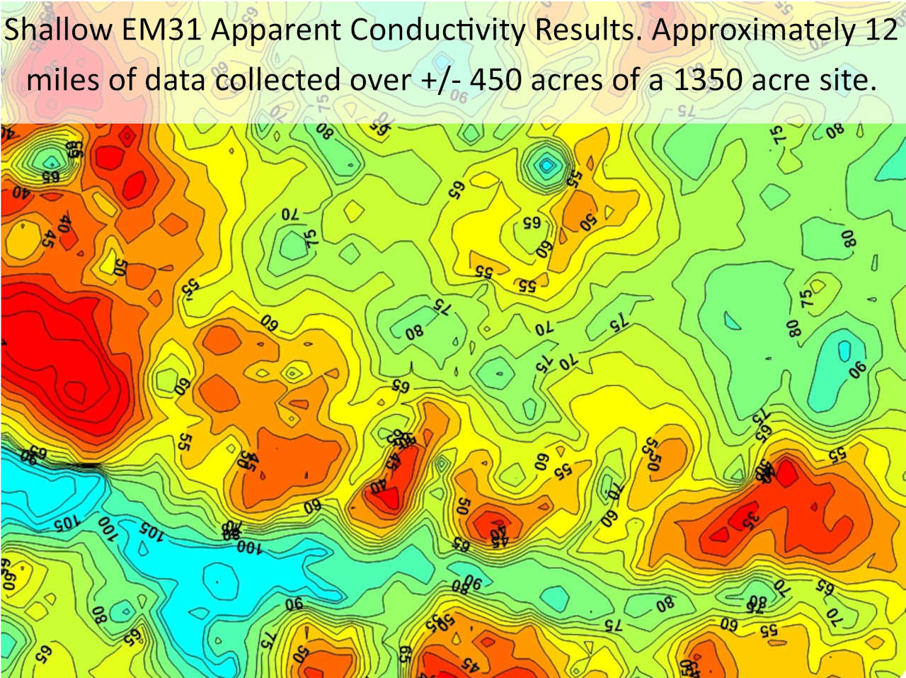
Electrical methods are one of the best ways to map out sand and gravel units. In contrast to bedrock surveys, the average depth of investigation needs to be limited to the overburden. If one penetrates too deep, then the response will be influenced by shallow bedrock conditions. The plot below is a smaller portion of a 1350 acre survey using a Geonics EM31. Lines were spaced approximately 200 to 250 feet apart. About 50 miles of line were walked over the 1350 acres. The purpose of the EM31 survey was to map sand and gravel units. Unlike electrical resistivity methods, low apparent conductivities are often associated with sand and gravel, assuming other factors remain constant.
Geonics EM31 Apparent Conductivity Plot 450 Acres
After the area was test pitted, areas colored red or yellow correlated well with about 10 to 15 feet of sand and gravel. Areas shaded blue, representing apparent conductivities over 100 mS/m, are nearly all clay. The areas shaded yellow-blue are transitional and represent a mixture of sand, gravel, and clay. Other portions of the site, not shown in this plot, indicated large tracks of land that were clay rich. Since retention ponds are being built by mining the sand and gravel, some of the clay will be redistributed to line the ponds. While sand and gravel units often have apparent conductivities below 10 mS/m, the top soil was very conductive at this site. The conductive top soil effectively increased the apparent conductivity of the bulk volume of material sampled by the EM31.
Locating trenches, excavations, fill, and tiles
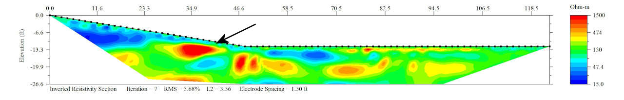
Investigations for trenches, excavations, fill, and tiles can be difficult depending on how much area is disturbed or the type of fill. Although GPR can locate tile lines with good site conditions, it may have a difficult time in areas with clay rich soils. MASW is the only cost effective seismic method that can map lateral variations in soil conditions. As previously noted, MASW is sensitive to changes in the stiffness of soils. The materials (e.g. sand verses clay) are not the only factors that control the stiffness of the soils. To some degree, the level of compaction influences shear wave velocities. Thus, trenches, excavations, and fill may be characterized using MASW. However, electrical methods offer some of the greatest detail. Below is a plot showing a gravel filled trench at the base of a hill. The arrow points to the trench, which is delineated by the high resistivity anomaly.
Electrical resistivity tomography images a trench located along the bottom of a hill.
The results represent one of thirty-five lines. The lines were acquired with an AGI 84 electrode SuperSting R8 system. To obtain this level of detail, the electrodes were placed one foot apart. They are represented on the diagram as small dots across the top of the plot. As a result, it took many days to detail the trench across the site. As seen, the electrical resistivity cross-section yielded other areas shaded red. While these red areas represented naturally occurring pockets of sand and/or gravel, they failed to map between resistivity lines and were less of a concern.
Geophysical characterizing weathered zones and karst void spaces
Ahh karst. One could dedicate an entire talk on karst. This topic covers a wide variety of conditions. Because karst environments range from inches to hundreds of feet in size, often take a very elusive path, and maybe unsaturated, saturated, or filled with soils, clearly one needs to define the size and depth of karst features before attempting to identify them. Although clients often look for depressions in the shallow bedrock surface, karst activity commonly falls along faults and joints. Thus, it is sometimes beneficial to map spatially large anomalies along linear features that suggest the presence of a fault. As a result, geophysical investigations focused on detecting or delineating karst features often incorporate all the methods discussed in this talk.
Characterizing fractures, joints, and faults
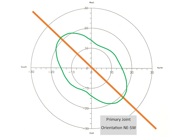
Geophysical methods, under good site conditions, map joints and faults. Fault zones and joint patterns created by faults can extend for miles. Highly weathered joints and faults are promising targets for geophysical methods. In contrast, smaller scale joint systems are more of a challenge. Nonetheless, the cumulative effect of more subtle joint systems is frequently observed in an azimuthal resistivity survey. On a large scale, a rock unit with joints is no longer isotropic. It is anisotropic. The secondary porosity created by a joint system produces a low resistance path for electricity to flow. By rotating a four pin Wenner array about a center point, one maps the apparent resistivity as a function of its orientation or its azimuth. Below are the post processed electrical resistivity results of an azimuthal resistivity survey.
Azimuthal Resistivity Joint Orientation NE-SW
In comparison to these results, a site with little or no detectable joints appears uniform or isotropic. Hence, the apparent resistivity values are the same for all orientations. The plotted data creates a circle. On the other hand, as jointing increases, the rock unit becomes more anisotropic. The effects impact the apparent electrical resistivity values. As one can observe here, the results did not yield a circle, they produced more of an ellipse, which is the theoretical shape for a single set of joints. The orange line on this diagram approximates the long axis of the crudely shaped ellipse. The orientation of this line is interpreted to reflect the orientation of the joints at depth.
Summary of geophysical methods for characterizing shallow bedrock
Unlike more deeply buried bedrock, geophysically investigating shallow rock is considerable less difficult. By all means, one can come up with shallow bedrock conditions that are more complicated. However, the ability to detect and map smaller features improves as the overburden thickness decreases. While cost can be an issue, I find there is seldom an investigation that a person can depend on only one geophysical method. There may be a primary geophysical approach but there is often one or more other methods supplementing the primary method, which improves the level of confidence in the final interpretation. Also, for those who conduct drilling programs, borings are a critical part of any comprehensive geophysical investigation. Boring logs assist with processing the geophysical results and provide a way to ground truth the interpretation, which may need to be modified over time as additional information is gathered.
Once again I thank the Wisconsin Association of Professional Agricultural Consultants for the opportunity to give this presentation.
This talk was presented by Arthur Fromm of Geophysical Services LLC a full service geophysical consulting company 262-242-4280. Geophysical equipment is available through his company K. D. Jones Instrument Corp., which rents geophysical equipment 262-442-6327.
Follow this link or go to the menu and click on the tab for geophysical services.
Locating Deep Facilities Using ERI, EM, MASW, pulseEKKO Ultra GPR, and Magnetometers for Buried Cables Voids Pipes
Geophysics for voids under buildings, floors, foundations, parking lots, and factories
Geophysical Services Conducted. A Short List of Clients, Landfills, Government Sites, and Locations.

Chart Comparing 57 Geophysical Methods With 17 Applications and Disciplines
Less Common Near Surface Geophysical Equipment
NAICS and SIC Codes for Geophysical Surveying and Mapping Services
Geophysics and Geophysical Services From Archives and Old Posts